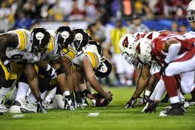
Sunday, June 8, 2014

Infinite Field Football

by Michael Nahas


Physicists are always talking about ideal environments, like infinite planes with zero friction. What if we extended that to football and had teams play on an infinite field with an infinite clock?

How would it work? One team would start with the ball, drive some number of yards down field, and then turn the ball over to the other team. At that point, the other team would take the ball, drive some amount of yards in the other direction, before turning the ball over to the first team. And so on.

They would go back and forth, except for one strange exception. That exception is when the ball carrier is the fastest guy on the field and he gets through the defense. Can he run for infinity? The short answer is yes. But, for the moment, let's assume that doesn't happen and, later, I'll tell how to handle when it does.

It's pretty obvious that "winning" on the infinite field means that your team, when it possesses the ball, moves the ball further than when the other team possesses it. So, the thing we want to compute is the expected length of a drive.

The most informative way to calculate that is to break the drive into series of downs. Each series either ends in a new first down or a turnover. So let's define:
P = probability of a series ending in a new first down
D1 = expected length of series that ends in a new first down
D4 = expected length of a series that doesn't end in a first down

Now, we can build an equation for the expected length of a drive by looking at the number of first downs that occurred in it.

Exactly 0 first downs occurs (1-P) of the time
Exactly 1 first downs occurs P*(1-P) of the time
Exactly 2 first downs occurs P*P*(1-P) of the time
...
Exactly N first downs occurs P^N*(1-P) of the time

In probability, this is the geometric distribution. The Wikipedia page gives us the mean: P/(1-P). (NOTE: if you check the Wikipedia page, they're answer is (1-p)/p. This because their p is equal to my 1-P.) Now, knowing the number of first downs, we can write the expected length of a drive:

Expected length of a drive = (P/(1-P))*D1 + D4

Now, suddenly, P becomes very interesting. As it gets bigger, the length of the drive grows faster than linear.

P=.75 ---> Expected first downs = 3
P=.80 ---> Expected first downs = 4
P=.85 ---> Expected first downs = 5.666

Regarding the other factors, I don't expect the "expected distance to a new first down" to vary much between teams. Team with better offenses will produce more yards but some of those yards will go to reaching the first down in fewer downs. The "expected distance without a first down" will probably only differ between teams that punt after 3 downs and those who "go for it" on fourth.

When should a team "go for it"? Well, there we need to know the chance of making a first down. If that times the expected length of drive is longer than your punt, the team should go for it. Teams that "go for it" on fourth will have a larger probability of getting a first down, which we saw above, is the key metric in infinite field football.

What does this mean to finite field football?
The first conclusion to draw is that first down percentage and drive length are key stats to look at. We all knew they were important before, but I think they are worth considering as _the_ team metrics to look at. Likewise, for defenses, their affect on first down percentage is important.

My second conclusion is that first down percentage has a non-linear affect on drive length. A lot of analysis techniques assume linear relationships between terms. We need to be careful about how we apply those techniques.

My third conclusion is actually a supposition. I believe that EPA by field position is based on the Ps of the two teams. Brian Burke in 2008 said it wasn't linear. The graph he produced was based on data for all teams, but he also said "Another complication is that various teams have different curves." I think with Ps, we can determine what EPA by field position should look like from a theoretic point of view.

What no data?
This post doesn't have any data. I spend my days programming, so that muscle is exhausted when I have time off. So, if you like the idea, I'd love to see data too.

If we took a team's downs between their own 10 and the opponent's 20, I think we'd see some clear trends. Monte carlo techniques at the series-of-downs level (or at the down-by-down level) could be used to estimate the length of drives. Long plays that resulted in touchdowns (that is, those infinite runs on the infinite length field) could be sidestepped by computing the median length of drive rather than the expected. I'll be interested to see if the data is significant enough to measure differences.

Another important thing to measure is the finite field aspects. How well does an estimate of performance on an infinite field predict performance inside your own 10 and inside their 20? Brian Burke in 2008 said that QBs weren't statistically significantly better (or worse) inside the red zone. Good outside was good inside. Is that true for the whole offense? If so, I think the infinite field model is worth keeping around.


Tuesday, January 7, 2014

How does weather affect a QB's QBR

By Krishna Narsu

A few years ago when I interned with ESPN, I had the pleasure of meeting the ESPN Analytics team. This was back when Total QBR was first being rolled out. After listening to a presentation the team gave on QBR, I became a fan of the metric. One of the things I was curious about was how weather impacted QBR. Does QBR go up in domes? Does QBR go down when it’s really cold? Dean Oliver, one of the creators of the statistic, was nice enough to send me the QBR data and I obtained the weather data by scraping the NFL gamebooks. I completed the study a few years ago but never thought of posting the results. Now, with the Green Bay-SF game expected to be bone-chillingly cold, I'm putting this post out.

When I conducted the study, I used an ANOVA to test if two samples of different weather data were significantly different. For example, one of the tests was rain
vs. no rain. I looked at a number of different categories: rain, hot/cold, wind, wind chill, domes, etc. Here were the results:


Monday, December 9, 2013

EP forfeited

Picture the scene. It’s February 2, 2014. We’re at the MetLife Stadium for Superbowl XLVIII. The opening kickoff has just gone for a touchback and out trots the offense. It’s first-and-ten. Here’s the snap and….

What the heck? The QB just spiked it. What a bizarre play call from the coach. It’s now second-and-ten. What is going on? Is the coach deliberately trying to lose this game?

Some time not much later in the game, with the score still tied, the coach faces fourth-and-two from the opponents 25. Out trots the field goal unit to attempt to give them the lead. “The field goal here is the right call”, proclaims Aikman. “You need to get points on the board. You don’t want to risk going for it and not coming away with something”

I’m sure you know where this is going. The opening spike, which would have been rightly called as crazy by everyone watching, cost the team 0.48 expected points. The field goal attempt, which would have been hailed as a no-brainer by the standard voices, cost them an almost identical 0.49 EP over going for it.

I got thinking about this after seeing a response to this tweet from the 4th Down Bot


In reply, @MattSantaMaria confidently stated that fractional points aren’t possible. Please go away and try again.

To be fair to him, he’s not wrong. Stating that a team cost themselves half a point is almost meaningless to someone who doesn’t have a grasp of probability. Explaining that attempting the field goal is as damaging to a team’s chances of winning as spiking the ball on the opening play of the game, however, might be more comprehensible.

Some other ‘crazy decision’ EP equivalents

  • Taking a deliberate delay-of-game penalty on third-and-five costs around 0.4 EP
  • Accepting an offside penalty when you’ve just gained 15 yards on a first-and-twenty play costs around 0.2 EP
  • Taking a knee on a second-and-five would cost around 0.65 EP


Tuesday, November 5, 2013

Should Colts have gone for 2

by Ian Simcox
So there I am, browsing my Twitter feed and I see this


Predictably the replies featured people as sure of the value of kicking the XP as Brian was of going for the 2.

At a 45% success rate on the 2-pts, the WP calculator says Indy have a 0.10WP if they kick the XP, comparing favourably to 0.09WP if they go for it (0.12 on success, 0.07 on failure). So, marginally the XPers have it. I must admit though, I plugged starting the 4th qtr down 10, 11 and 12 on 1st down into the calculator, to simplify the second part of this article.

What really interests me is the uncertainty around these numbers, which is always important on these tight calls. The XPers may have it on the WP calculator, but if those numbers are +/- 0.03WP then it’s impossible to say which is right.


Saturday, November 2, 2013

The Colts and their New “Run-Heavy” Offense

By Sal Cacciatore

When the Indianapolis Colts hired Pep Hamilton to be their offensive coordinator in January, the team’s buzzword this past offseason was “balance,” with coaches stressing the need to run the ball to win.

While that may be cringe-worthy for anyone familiar with this site and Brian’s work on the topic, the Colts stand at 5-2, so there is a sentiment of vindication for Hamilton and head coach Chuck Pagano’s conservative coaching. Mike Wells of ESPN.com, formerly of the Indianapolis Star, went as far as to say the team “got their record by being a run-first team.”

Leaving aside how foolish molding a team led by prodigal quarterback Andrew Luck into a “run-first” club seems, we can use numbers to assess if Wells’ statement and others like it are true.

Are the Colts actually a run-based team and are they winning because of a newfound emphasis on running?


Friday, October 18, 2013

NFL Team snapshots - Week 6

by Tom McDermott
(This submission of a repost and can be found at its original home here. ED)

I've added a few more things to the Snapshots this week, namely, correlation values. I thought it might be interesting to see how the various Expected Points totals correlate with Margin of Victory and Win Percentage. For those of you unfamiliar with correlation (I know I was until I started getting into all this stat stuff): a correlation of 1.0 is perfect correlation, a correlation of 0.0 is no relationship. As far as Win Percentage, it makes sense that the offense and defense EPA correlations are the same - the way EPA works, for every point gained on offense, there is a point lost on defense (or vice versa). But I was surprised to see the higher Special Teams correlation. I'm not sure this means anything yet - the numbers will most likely regress as the season goes on. But it is interesting to note that the top three teams in terms of Margin of Victory - Denver, Kansas City, and Seattle - also have the top three special teams EPA scores.


Conversion percentage VS win percentage

by Andy Steiner


The intent of this study is to see how much more likely strong teams are to convert third or fourth downs compared to weak teams.

In this study I plot various conversion probabilities of 3rd and 4th downs, as a function of team strength (and distance to go). The measure of team strength that I use is the offense’s end of season winning percentage minus the defense’s end of season winning percentage. For the purpose of this study offensive conversion percentage is the number of times a team coverts a third and fourth down divided by the number of attempts to make that conversion. And of course the defensive conversion percentage is the number of times the defense holds on third and fourth down divided by the number of attempts.
So my X and Y variables are:

X =(Offense end of season winning percentage) – (Defense end of season winning percentage)

Y = 1 (successful conversion or TD), 0 (failed conversion)

I know there are much better ways to measure how good an offense or defense is than the end of season winning percentage; but I think this is a good first step. I also think it’s accessible. If a coach wants to get a better idea of how likely they might be to convert in a certain situation the win-loss records might be the first thing they think of. It’s probably how they think of their team strength – “we are a 12 and 4 team”.
I then plot a linear fit from all the 1 and 0 y data points. This means I am assuming that the “true” probability of conversion is a linear function of team W-L record.

I use data from 2002 to 2011 (regular season plus playoffs). I use most of the “normal football” assumptions, but not all. I was slightly more aggressive with time, allowing the 2nd quarter to be counted all the way up to 7 minutes left. The 4th quarter is excluded; all of the 1st and 3rd quarters are included. The plays are only included if the line of scrimmage is between a team’s own 25 and the opponents 20. The score differential is limited to 10 points.